Storing data¶

When storing data, we have two main requirements: 1. We want to be able to store n-dimensional data structures. 2. The data structures must be self-explanatory, that is, they must contain sufficient information to draw a basic plot of the data.

.. _sampled_plot:

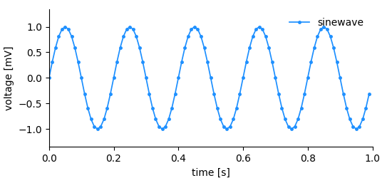
Considering the simple plot above, we can list all information that it shows and by extension, that needs to be stored in order to reproduce it.

the data (voltage measurements)
the y-axis labeling, i.e. label (voltage) and unit (mV)
the x-axis labeling, i.e. label (time) and unit (s)
the x-position for each data point
a title/legend

In this, and in most cases, it would be inefficient to store x-, and y-position for each plotted point. The voltage measurements have been done in regular (time) intervals. Thus, we rather need to store the measured values and a definition of the x-axis consisting of an offset, the sampling interval, a label, and a unit.

This is exactly the approach chosen in NIX. For each dimension of the data a dimension descriptor must be given. In NIX we define three dimension descriptors:

SampledDimension: Used if a dimension is sampled at regular intervals.
RangeDimension: Used if a dimension is sampled at irregular intervals. The instances at which the data has been sampled are stored as ticks. These ticks may also be stored in a DataArray or DataFrame, the Range Dimension can link to it.
SetDimension: Used for dimensions that represent categories rather than physical quantities.

The DataArray¶

The DataArray is the most central entity of the NIX data model. As almost all other NIX-entities it requires a name and a type. Both are not restricted but names must be unique within a Block. type information can be used to introduce semantic meaning and domain-specificity. Upon creation, a unique ID will be assigned to the DataArray.

The DataArray stores the actual data together with label and unit. In addition, the DataArray needs a dimension descriptor for each data dimension. The following snippet shows how to create a DataArray and store data in it.

Storing data in a DataArray (example code).¶

    data = block.create_data_array("sinewave", "nix.regular_sampled", data=y,
                                   label="voltage", unit="mV")
    # add a descriptor for the xaxis
    data.append_sampled_dimension(stepsize, label="time", unit="s", offset=0.0)

As promised, the DataArray contains all information to create a basic plot (see the figure above).

    x_axis = data_array.dimensions[0]
    x = x_axis.axis(data_array.data.shape[0])
    y = data_array.data[:]

    plt.plot(x, y, marker=".", markersize=5, label=data_array.name)
    plt.xlabel(x_axis.label + " [" + x_axis.unit + "]")
    plt.ylabel(data_array.label + " [" + data_array.unit + "]")
    plt.xlim(0, np.max(x))
    plt.ylim((1.1 * np.min(y), 1.1 * np.max(y)))
    plt.legend()
    plt.show()

The highlighted lines emphasize how information from the dimension descriptor (a SampledDimension) and the DataArray itself are used for labeling the plot.

In the example shown above, the NIX library will figure out the dimensionality of the data, the shape of the data and its type. The data type and the dimensionality (i.e. the number of dimensions) are fixed once the DataArray has been created. The actual size of the DataArray can be changed during the life-time of the entity.

In case you need more control, DataArrays can be created empty for later filling e.g. during data acquisition.

data_array = block.create_data_array("sinewave", "nix.sampled", dtype=nixio.DataType.Double, shape=(100));

The resulting DataArray will have an initial size (100 elements) which will be automatically resized, if required. The data type is set to nixio.DataType.Double. The NIX library will further try to convert passed data to the defined data type, if possible. Note: Data type and rank (i.e. the number of dimensions) cannot be altered after the DataArray has been created.

Data is then set by calling

array.write_direct(voltage)

Data is read from a DataArray by accessing it in numpy style.

# read the full data
data = array[:]

# reading only the first 100 points
data = array[:100]

# replacing data
array[:100] = np.zeros(100)

DataArrays can also be extended by appending data.

array = block.create_data_array("test data", "test", data=np.random.randn(100))
print(array.shape)
array.append(np.ones(100))
print(array.shape)

Dimensions¶

Within the DataArray we can store n-dimensional data. For each dimension we must provide a dimension descriptor. The following introduces the individual descriptors.

SampledDimension¶

Here we have the same situation as before, the data has been sampled in regular intervals. That is, the time between successive data points is always the same. The x-axis can be fully described with just a few parameters:

sampling interval
offset
label
unit

The SampledDimension entity is used in such situations and needs to be added to the DataArray entity upon creation:

A dimension in which the data has been gathered in regular intervals is described using a SampledDimension (example code¶

    data = block.create_data_array("sinewave", "nix.regular_sampled", data=y,
                                   label="voltage", unit="mV")
    # add a descriptor for the xaxis
    data.append_sampled_dimension(stepsize, label="time", unit="s", offset=0.0)

SetDimension¶

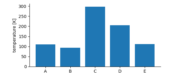
If we need to store data that falls into categories, i.e. the x-positions are not numeric or the dimension does not have a natural order, a SetDimension is used. It stores a label for each entry along the described dimension.

A categorical data dimension is described with a SetDimension which (optionally) stores labels for each category (example code)¶

    data_array = b.create_data_array("category data", "nix.categorical", data=data, label="temperature", unit="K")
    data_array.append_set_dimension(categories)

RangeDimension¶

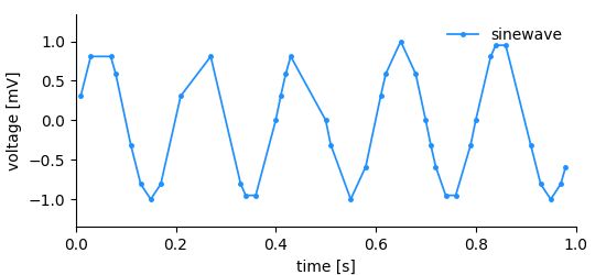
A signal similar to what we had before is recorded but this time the temporal distance between the measurements is not regular. Storing this kind of data is not as efficient as in the regularly sampled case since we need to store the time of each measurement and the measured value. The following information needs to be stored to describe the dimension:

x-positions of the data points, i.e. ticks
label
unit

In this kind of dimension we store a range of ticks, therefore the name RangeDimension. It needs to be added to the DataArray when it is created.

Storing irregularly sampled data (example code).¶

    times, values = create_data(1.0, 0.02)

    # create a new file overwriting any existing content
    file_name = 'irregular_data_example.nix'
    file = nixio.File.open(file_name, nixio.FileMode.Overwrite)

    # create a 'Block' that represents a grouping object. Here, the recording session.
    block = file.create_block("block name", "nix.session")

    # create a 'DataArray' to take the data, add some information about the signal
    data = block.create_data_array("sinewave", "nix.irregular_sampled", data=values,
                                   label="voltage", unit="mV")
    # add a descriptor for the xaxis
    data.append_range_dimension(ticks=times, label="time", unit="s")

Note: The ticks of a RangeDimension must be numeric and ascending.

The RangeDimension can do more. Consider the case that the times of an event are stored:

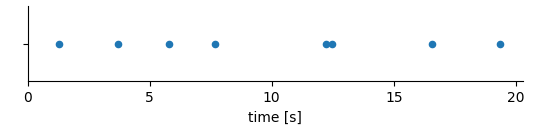
For example these might be the times of action potentials (aka spikes) recorded in a nerve. In such a case it is basically the x-values that are of interest. It would be inefficient to store them twice, first as values in the DataArray and then again as ticks in the dimension descriptor. In such cases the RangeDimension is set up to link to the DataArray itself.

A RangeDimension can link to a DataArray as a source of the ticks (exmaple code).¶

    event_times = create_data(10., 1.0)
    nixfile = nixio.File.open("range_link.nix", nixio.FileMode.Overwrite)
    b = nixfile.create_block("session", "nix.session")

    data_array = b.create_data_array("event times", "nix.event.times", data=event_times, label="time", unit="s")
    data_array.append_range_dimension_using_self()

In the highlighted line we use a convenience function to establish the link between the dimension descriptor and the data stored via the dimensions of its own DataArray.

This function is a shortcut for:

rdim = data_array.append_range_dimension()
rdim.create_link(data_array, index=[-1])

In the same way one can set up the RangeDimension to use a DataFrame. The index defines which slice of the data stored in the DataArray/Frame holds the ticks. The slice must be a 1-D vector within the linked data. If, for example, the DataArray is 2-D and the ticks are in the 3rd column then the index would be [-1, 3]. The -1 marks the dimension along which to look for the ticks. When linking DataFrames the index notes the column.

Advanced storing¶

Data compression¶

By default data is stored uncompressed. If you want to use data compression this can be enabled by providing the nixio.Compression.DeflateNormal flag during file-opening:

import nixio
f = nixio.File.open("test.nix", nixio.FileMode.Overwrite, compression=nixio.Compression.DeflateNormal)

By doing this, all data will be stored with compression enabled, if not explicitly stated otherwise. At any time you can select or deselect compression by providing a nixio.Compression flag during DataArray creation. Available flags are:

nixio.Compression.Auto: compression as defined during file-opening.
nixio.Compression.DeflateNormal: use compression (fixed level).
nixio.CompressionNo: no compression.

data_array = b.create_data_array("some data", "nix.sampled", data, compression=nixio.Compression.DeflateNormal);

Note the following:

Compression comes with a little cost of read-write performance.
Data compression is fixed once the DataArray has been created, it cannot be changed afterwards.
Opening and extending a compressed DataArray is easily possible even if the file has not been opened with the nixio.Compression.DeflateNormal flag.

Supported DataTypes¶

DataArrays can store a multitude of different data types. The supported data types are defined in the nixio.DataType enumeration:

nixio.DataType.Bool: 1 bit boolean value.
nixio.DataType.Char: 8 bit charater.
nixio.DataType.Float: floating point number.
nixio.DataType.Double: double precision floating point number.
nixio.DataType.Int8: 8 bit integer, signed.
nixio.DataType.Int16: 16 bit integer, signed.
nixio.DataType.Int32: 32 bit integer, signed.
nixio.DataType.Int64: 64 bit integer, signed.
nixio.DataType.UInt8: 8 bit unsigned int.
nixio.DataType.UInt16: 16 bit unsigned int.
nixio.DataType.UInt32: 32 bit unsigned int.
nixio.DataType.UInt64: 64 bit unsigned int.
nixio.DataType.String: string value.
nixio.DataType.Opaque: data type for binary data.

The data type of a DataArray must be specified at creation time and cannot be changed. In many cases, the NIX library will try to handle data types transparently and cast data to the data type specified for the DataArray in which it is supposed to be stored.

Extending datasets on the fly¶

The dimensionality (aka rank) and the stored DataType of a DataArray are fixed. The actual size of the stored dataset, however, can changed. This is often used when you acquire data continuously e.g. while recording during an experiment. In nixpy the resizing is handled transparently.

The workflow would be:

Preparations: Open a nix-file in nixio.FileMode.ReadWrite or nixio.FileMode.Overwrite. Create or open the DataArray.
Acquire more data.
Append the acquired data to the data array.
Acquire more data.

The following code shows how this works.

Extending DataArray size e.g while recording continuously (example code)¶

    nixfile = nixio.File.open("continuous_recording.nix", nixio.FileMode.Overwrite, compression=nixio.Compression.DeflateNormal)
    block = nixfile.create_block("Session 1", "nix.recording_session")
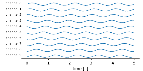
    data_array = block.create_data_array("multichannel_data", "nix.sampled.multichannel", dtype=nixio.DataType.Double,
                                         shape=(chunk_samples, number_of_channels), label="voltage", unit="mV")
    data_array.append_sampled_dimension(0.001, label="time", unit="s")
    data_array.append_set_dimension(labels=["channel %i" % i for i in range(number_of_channels)])

    chunks_recorded = 0
    while chunks_recorded < number_of_chunks:
        data = record_data(chunk_samples, number_of_channels, dt)
        if chunks_recorded == 0:
            data_array.write_direct(data)
        else:
            data_array.append(data, axis=0)
        chunks_recorded += 1
        print("recorded chunks %i: array shape %s" % (chunks_recorded, str(data_array.shape)))

Note! Selecting the initial shape defines the chunk size used to write the data to file. Choose it appropriately for the expected size increment. Selecting a size that is too small can severly affect efficiency.

The DataFrame¶

The DataFrame stores tabular data in a rows-and-columns format. Each Column has a name, a data type, and, optionally, a unit and a definition.

A DataFrame is created by providing the column definition which consists of a name and the data type that should be stored in each column. Units can be added later on. It is best to use OrderdDicts to make sure, that the column order is as defined (standard dictionaries do not guarantee the order of the items). example code¶

    block = nixfile.create_block("test block", "recordingsession")
    column_definitions = OrderedDict([('name', str), ('id', str), ('time', float),
                                      ('amplitude', np.float64), ('frequency', np.float64)])

    column_units = ["", "", "s", "mV", "Hz"]
    column_data = [("alpha", nixio.util.create_id()[:10], 20.18, 5.0, 100),
                   ("beta", nixio.util.create_id()[:10], 20.09, 5.5, 101),
                   ("gamma", nixio.util.create_id()[:10], 20.05, 5.1, 100),
                   ("delta", nixio.util.create_id()[:10], 20.15, 5.3, 150),
                   ("epsilon", nixio.util.create_id()[:10], 20.23, 5.7, 200),
                   ("fi", nixio.util.create_id()[:10], 20.07, 5.2, 300),
                   ("zeta", nixio.util.create_id()[:10], 20.12, 5.1, 39),
                   ("eta", nixio.util.create_id()[:10], 20.27, 5.1, 600),
                   ("theta", nixio.util.create_id()[:10], 20.15, 5.6, 400),
                   ("iota", nixio.util.create_id()[:10], 20.08, 5.1, 200)]

    data_frame = block.create_data_frame("test data frame", "signal1",
                                         data=column_data, col_dict=column_definitions)

For a quick overview one can use the DataFrame.print_table() method

column:     name       id       time   amplitude frequency
unit:                          s         mV        Hz
[0]:    alpha   e28e0735-1  20.18      5.0      100.0
[1]:     beta   74942839-1  20.09      5.5      101.0
[2]:    gamma   0886ef1a-2  20.05      5.1      100.0
[3]:    delta   0ac53fd2-7  20.15      5.3      150.0
[4]:   epsilon  a54b35df-1  20.23      5.7      200.0
[5]:      fi    70eb952c-0  20.07      5.2      300.0
[6]:     zeta   130ad527-d  20.12      5.1       39.0
[7]:     eta    042a460c-e  20.27      5.1      600.0
[8]:    theta   1f2c1df8-f  20.15      5.6      400.0
[9]:     iota   c4598a1e-b  20.08      5.1      200.0

The DataFrame offers several methods to get basic information about the table:

    print("size, aka number of rows: ", data_frame.size)
    print("column names: ", data_frame.column_names)
    print("column definition: ", data_frame.columns)
    print("column units: ", data_frame.units)

Leading to the following output:

size, aka number of rows:  10
column names:  ('name', 'id', 'time', 'amplitude', 'frequency')
column definition:  [('name', dtype('O'), None), ('id', dtype('O'), None), ('time', dtype('<f8'), 's'), ('amplitude', dtype('<f8'), 'mV'), ('frequency', dtype('<f8'), 'Hz')]
column units:  [None None 's' 'mV' 'Hz']

Reading of the table data is possible for individual cells, entire columns, or selected rows

    print("single cell by position: ", data_frame.read_cell(position=(0, 0)))
    print("single cell by name and row index: ", data_frame.read_cell(col_name="name", row_idx=[0]))

    print("Entire ID column: ", data_frame.read_columns(name="id"))
    print("Two columns, id and name, joined: ", data_frame.read_columns(name=["id", "name"]))

    print("Entire rows with indices 0 and 2: ", data_frame.read_rows([0, 2]))

Which yields the following outputs:

single cell by position:  alpha
single cell by name and row index:  alpha
Entire ID column:  ['f0299d50-b' 'c74d3b7c-0' 'e27bb6f7-2' '8bac251b-7' 'aecc18d4-a'
'268c8dea-f' '88de352a-d' '4bdac82c-b' '5671ed6e-b' '0a7bf5e4-9']
Two columns, id and name, joined:  [('f0299d50-b', 'alpha') ('c74d3b7c-0', 'beta') ('e27bb6f7-2', 'gamma')
('8bac251b-7', 'delta') ('aecc18d4-a', 'epsilon') ('268c8dea-f', 'fi')
('88de352a-d', 'zeta') ('4bdac82c-b', 'eta') ('5671ed6e-b', 'theta')
('0a7bf5e4-9', 'iota')]
Entire rows with indices 0 and 2:  [('alpha', 'f0299d50-b', 20.18, 5. , 100.)
('gamma', 'e27bb6f7-2', 20.05, 5.1, 100.)]