Image data
Color images can be stored as 3-D data in a DataArray. The first two dimensions represent width and height of the image while the 3rd dimension represents the color channels. Accordingly, we need three dimension descriptors. The first two are SampledDimensions since the pixels of the image are regularly sampled in space. The third dimension is a SetDimension with labels for each of the channels. In this tutorial the “Lenna” image is used. Please see the author attribution in the code.
example code , the 
image imagemagick or xv packages).¶ data = block.create_data_array("lenna", "nix.image.rgb", data=img_data)
# add descriptors for width, height and channel dimensions
data.append_sampled_dimension(1, label="height")
data.append_sampled_dimension(1, label="width")
data.append_set_dimension(labels=channels)

Tagging regions
One key feature of the nix-model is its ability to annotate, or “tag”, points or regions-of-interest in the stored data. This feature can be used to state the occurrence of events during the recording, to state the intervals of a certain condition, e.g. a stimulus presentation, or to mark the regions of interests in image data. In the nix data-model two types of Tags are discriminated. (1) the Tag for single points or regions, and (2) the MultiTag to annotate multiple points or regions using the same entity.
Tagging a single point or region
Single points of regions-of-interest are annotated using a Tag object. The Tag contains the start position and, optional, the extent of the point or region. The link to the data is established by adding the DataArray that contains the data to the list of references. It is important to note that position and extent are arrays with the length matching the dimensionality of the referenced data. The same Tag can be applied to many references as long as position and extent can be applied to these.
singleROI.py).¶ position = [250, 250, 0]
extent = [30, 100, 3]
tag = block.create_tag('Region of interest', 'nix.roi', position)
tag.extent = extent
tag.references.append(data)

Tagging multiple regions
For tagging multiple regions in the image data we again use a MultiTag entity.
example code).¶ num_dimensions = len(data.dimensions)
roi_starts = np.zeros((num_regions, num_dimensions), dtype=int)
roi_starts[0, :] = [250, 245, 0]
roi_starts[1, :] = [250, 315, 0]
roi_starts[2, :] = [340, 260, 0]
roi_extents = np.zeros((num_regions, num_dimensions), dtype=int)
roi_extents[0, :] = [30, 45, 3]
roi_extents[1, :] = [30, 40, 3]
roi_extents[2, :] = [25, 65, 3]
# create the positions DataArray
positions = block.create_data_array("ROI positions", "nix.positions", data=roi_starts)
positions.append_set_dimension() # these can be empty
positions.append_set_dimension()
# create the extents DataArray
extents = block.create_data_array("ROI extents", "nix.extents", data=roi_extents)
extents.append_set_dimension()
extents.append_set_dimension()
# create a MultiTag
multi_tag = block.create_multi_tag("Regions of interest", "nix.roi", positions)
multi_tag.extents = extents
multi_tag.references.append(data)
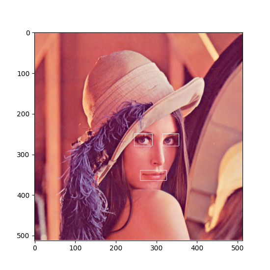
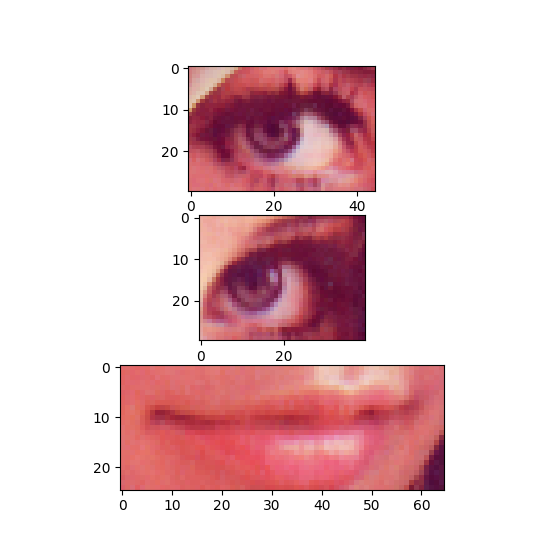
The start positions and extents of the ROIs are stored in two separate DataArrays, these are each 2-D, the first dimension represents the number of regions, the second defines the position/extent for each single dimension of the data (height, width, color channels).
The MultiTag has a tagged_data method that is used to retrieve the data tagged by the MultiTag.
tagged_data method. The first argument is the region number, the second the name of the referenced DataArray (example code).¶ roi_data = tag.tagged_data(p, "lenna")[:]
roi_data = np.array(roi_data, dtype='uint8')
ax = fig.add_subplot(position_count, 1, p + 1)
image = img.fromarray(roi_data)
ax.imshow(image)